Sampling - From Metropolis-Hastings, Hamiltonian MC to Langevin Dynamics

The more I use ChatGPT, the more I can feel the boost in learning efficiency. This blog is written by human but ChatGPT was used extensively to learn the concept of sampling. Now let's get into the topic - Sampling.

Why are we interested in sampling? You might have heard Langevin Dynamics in the score based generative modeling. But what the hell is Langevin Dynamics? Why do we need that? In this blog post, I will use mixture of gaussians distribution as an example to demonstrate how to draw samples from mixture of gaussians. Starting from Metropolis-Hastings to Hamiltonian MC and finally to Langevin Dynamics, we will get better understandings of these algorithms.

Problem Statement

Suppose you have a mixture of 2D gaussians:

$p(x) = \sum_{i=0}^{k}{\frac{1}{2\pi}det(\Sigma_i)^{-\frac{1}{2}}exp(-\frac{1}{2}(x-\mu_i)^T\Sigma_{i}^{-1}(x-\mu_i))}$ and $x = [x_1, x_2] \in R^2$.

Here is the Python code for this distribution:

MIX_RATIO = torch.Tensor([0.1, 0.8, 0.1])
MEAN_VEC = torch.Tensor([[0.0, 0.0], [8.0, 8.0], [8.0, 0.0]])
VAR_VEC = torch.Tensor([[1.0, 4.0], [1.0, 1.0], [4.0, 1.0]])


def eval_gaussian(x, mean, var):
    """Evaluate a Gaussian distribution."""
    coeff = 1.0 / (2.0 * np.pi * torch.sqrt(torch.prod(var)))
    exp_value = torch.exp(-0.5 * torch.sum(torch.pow(x - mean, 2) / var))
    return coeff * exp_value


def mixture_of_gauss(x: torch.Tensor):
    prob = torch.tensor(0.0)
    for idx in range(len(MIX_RATIO)):
        prob += MIX_RATIO[idx] * eval_gaussian(x, MEAN_VEC[idx], VAR_VEC[idx])

    return prob

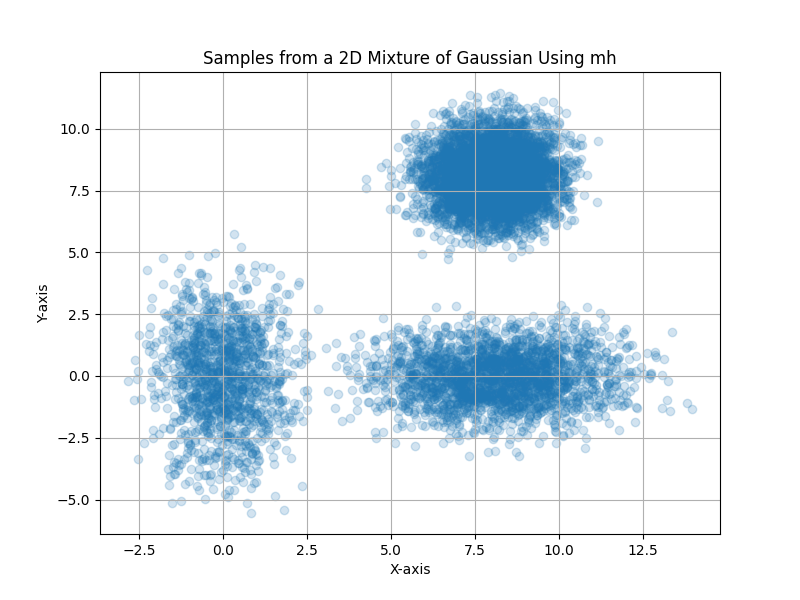
You can adjust the mix ratio, mean vector location and variance matrix (here I assume no covariance between $x_1$ and $x_2$). Now, use your imaginations, this distribution will have 3 modes at different centers and the one centered at $[8.0, 8.0]$ should have the largest weights.

Metropolis-Hastings (MH)

MH algorithm is a type of MCMC (Monte-Carlo Markov Chain) sampling method. The core idea of MCMC is to construct a markov chain process that can converge to the target distribution $\pi(x)$. In our example, the target distribution is a mixture of gaussian.

MH algorithm utilizes a proposal distribution and an acceptance procedure to determine if there should be state transitions. More details can be found in the Wikipedia.

def metropolis_hastings(steps=10000):
    # Use Gaussian as proposal distribution
    samples = torch.zeros((steps, 2))
    x_current = torch.Tensor([0, 0])

    i = 0
    while i < steps:
        x_proposal = x_current + torch.randn(2)
        p_current = mixture_of_gauss(x_current)
        p_proposal = mixture_of_gauss(x_proposal)

        # Acceptance criteria
        if p_proposal / p_current > np.random.rand():
            x_current = x_proposal
            samples[i] = x_current
            i += 1

    return samples

For Markov Chain, if the transition matrix satisfies detailed balance condition to a distribution $\pi(x)$ and is ergodic (basically means not trapped in cycles), the markov chain will eventually converge to its stationary distribution. It's also why we often see burn-in period that throws away the initial points. It tries to reduce the impact of the initial points.

Here are the example result of MH sampling:

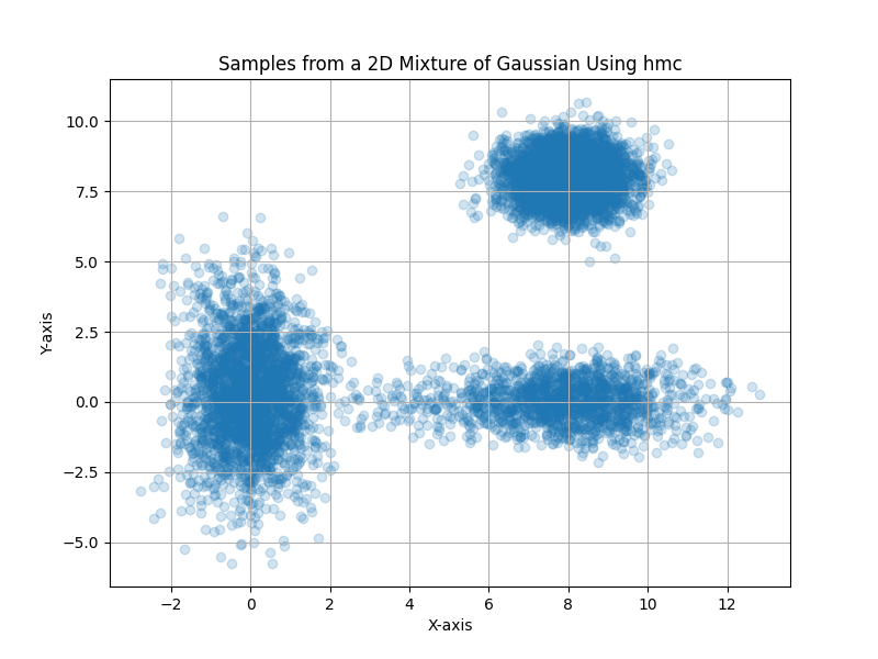
Hamiltonian Markov Chain

In the Metropolis-Hastings (MH), you may notice the samples between each step are correlated. The Gaussian random walk will not be able to move state too far away. Hamiltonian MC is proposed to allow the states to be moved further away. For distributions like mixture of gaussians, it is quite useful so the samples will not stuck in one of the modes. Similarly, more details can be found in the Wikipedia.

def hamiltonian_mc(steps, step_size, leapfrog_steps):
    samples = torch.zeros((steps, 2))
    current_q = torch.randn(2)
    i = 0
    while i < steps:
        q = current_q.clone()
        p = torch.randn(2)
        current_p = p.clone()

        # Leapfrog integration
        p -= step_size * grad_mixture_of_gauss(q.clone()) / 2
        for _ in range(leapfrog_steps):
            q += step_size * p
            p -= step_size * grad_mixture_of_gauss(q.clone())

        # Metropolis acceptance
        current_U = -torch.log(mixture_of_gauss(current_q))
        current_K = torch.sum(current_p**2) / 2
        proposed_U = -torch.log(mixture_of_gauss(q))
        proposed_K = torch.sum(p**2) / 2

        if np.random.rand() < torch.exp(current_U - proposed_U + current_K - proposed_K):
            current_q = q
            samples[i] = current_q
            i += 1

    return samples

Here are the results for HMC sampling:

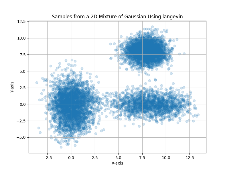
Langevin Dynamics

Finally, let's look into Langevin dynamics. After you see Hamiltonian MC, a natural thought would be "can we sample with other dynamics". And yes, researchers find that Langevin dynamics can also generate samples that converges to the target distribution. Compared to HMC, it does not involve the leapfrog integration, which can run faster. And compared to MH, it leverages the gradient of log-target-distribution that has potential to move states further. Now, let's look into the state transition equation:

$x_{t+1} = x_t + \epsilon \nabla_x logp(x) + \sqrt{2 \epsilon} z_t, z_t ~ N(0,1)$

The $\nabla_x logp(x)$ is the score function, and $\epsilon$ is the noise scale that we see from diffusion models.

def langevin_dynamics(steps, noise_scale):
    samples = torch.zeros((steps, 2))
    current_x = torch.randn(2, requires_grad=True)

    for i in range(steps):
        current_x.requires_grad_(True)
        p_x = torch.log(mixture_of_gauss(current_x))
        p_x.backward()

        with torch.no_grad():
            # Langevin dynamics step
            current_x = current_x + noise_scale * current_x.grad + np.sqrt(2 * noise_scale) * torch.randn(2)

        samples[i] = current_x

    return samples.detach().numpy()

Here are the results for Langevin dynamics sampling:

Lastly

You may think that all these methods give similar sampling results. But the actual number of iterations can be different (e.g. in this MH and HMC implementation, there are acceptance and rejection process that could increase the actual iterations). Also, the random seed is chosen that we can see all 3 modes of the gaussian. If you change the seed, sometimes Langevin dynamics only shows 2 modes of the gaussian (also known as mode collapse).

The full code is released in https://github.com/randxie/randxie.github.io/tree/master/code/sampling/main.py. Have fun.